
Logistic Regression in Python
Logistic Regression is one of the best classification algorithms of machine learning used for predictive analysis. This algorithm is mainly used for binary classification problems. This blog would help you to go through and understand all the below topics to understand logistic regression with a use case along with python.
- What is the difference between regression and classification
- Linear regression versus Logistic regression
- Logistic Regression
- Use cases of logistic regression
- Demo of logistic regression
- Evaluation of Logistic regression built.
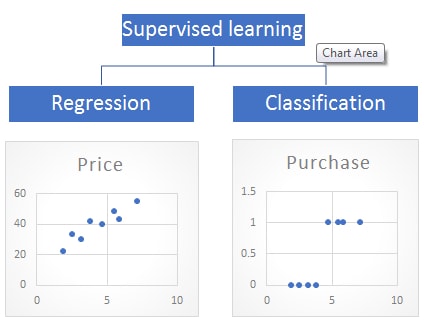
Difference between Regression and Classification:
Regression and classification come under the same umbrella of supervised machine learning algorithms. In supervised algorithms, we train the model using the labeled data (both input and output provided) and predict the output for the new data.
The major difference between regression and classification is that we use regression for predicting a numeric or continuous dependent (output) variable, but classification techniques are used for predicting the discrete or categorical dependent variable.
Linear regression vs Logistic regression:
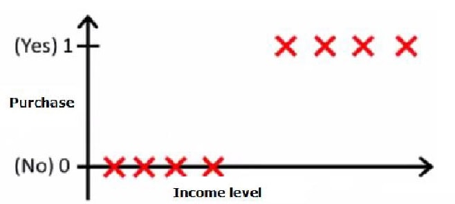
Linear regression is a machine learning algorithm used for solving regression problems and Logistic regression for classification. If so, why is a classification algorithm called a regression? And can classification be done using regression? Let us take an example of classification where you need to predict whether users purchase (binary 0-no purchase, 1-purchase) a certain product based on his income or not? When plotted data might look like below.
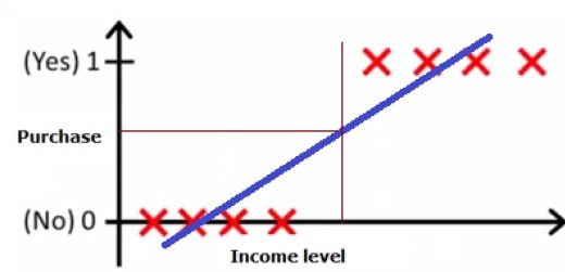
For this data above we can still fit the regression line like below, and still get the predictions.
But what if data is complex and the regression line can’t fit the data like below?
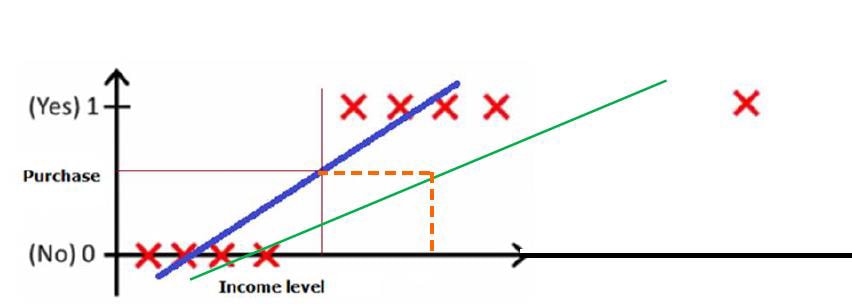
So instead of a regression line that we use to predict the data using linear regression, we need something else which can fit this discrete data, for accurate predictions of the dependent variable when it is categorical. Basically, like the graphs shown below

So the sigmoid curve comes as a savior for our problem, the sigmoid curve is one of the powerful tools in mathematics which can convert any value given to value between 0 and 1(probabilities).
Sigmoid curve equation is given below:
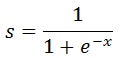
To convert the regression line to this sigmoid function we can use our regression equation in place of ‘x’ in the sigmoid function above.
But to refactorize the regression equation and give it a proper understandable meaning we need to use something called odds ratio which is said to be the ratio of the probability of winning to the probability of failure.

So, we observe that the regression output would be equal to log of odds of the probabilities, that’s why we call this machine learning algorithm as Logit or Logistic regression even if it is used for classification problems.
Types of logistic regression and use cases:
Even though the logistic regression is most used for predicting Binary categorical variable, it can also be used for predicting multiclass variables too, these below are three types of logistic regressions.
Binary Logistic regression:
When the dependent variable is a binary one which has classes of either 0 or 1, yes or No, True or False and High or low, then we use this type to solve such kind of problem.
Use case:
A bank is been suffering from the high churn rates in recent times and also loosing some high valued customers, the bank has all the personnel and financial data of customers with it, now it wants to know which customer has the max probability to churn and protect them by giving offers accordingly.
If we look into the above use case the dependent or the class variable that we will be dealing with would be “Whether customer churns or not” and has classes “Yes” or “No” so it’s a binary problem.
Ordinal Logistic (ordinal Multinomial) Regression:
When we want to predict a dependent variable that has a specific order(ordinal) in its classes and has more than two classes like high, medium and low.
Use case:
Let us take the same bank churn example, let us take that we have predicted the customers who are with a high probability of churn, but now the bank is not interested to give all offers to all customers to protect them. It wants to give offers based on the value (high, Low and med) of customers, so now we can make use of ordinal regression.
Nominal Logistic (Nominal Multinomial) Regression:
When we are dealing with the dependent variable that has no order (nominal) with multiple (three or more) classes then we can call it as nominal regression.
Use Case:
Suppose we want to build an AI camera based on image processing that can automatically predict the different pets (Dog, cat and other pets) entering an apartment and show their tag so that it would alert the security on it. Here just we are classifying the image to know what pet is entering, which doesn’t have any prominence attached to it.
Demo of logistic regression using python:
Use Case:
A car company is in a plan to introduce new kind of service plan to their customers, and they want to target high valued customers and offer them special offers along with the service plan and they have no interest in advertising their new product to save time and money when they know that there is no chance that a particular customer will not buy their product, so being data scientist we need to build a predictive model to say whether a customer is willing to purchase car companies service plan based on the user data.
Since the variable that we need to predict is binary (will purchase or not) we can make use of logistic regression to build the predictive model. Let us go through all the important stages for building a predictive model.
Data collection:
The first step of building a predictive model would be collecting the data, in this use case we have data on local disk, which is in CSV format. Let us load the data sets before performing some actions on it.
Note: All the python programming would be done using Jupiter notebooks.
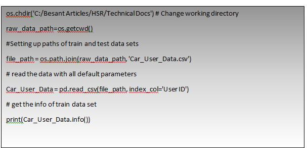
<class 'pandas.core.frame.DataFrame'> Int64Index: 400 entries, 15624510 to 15594041 Data columns (total 4 columns): Sex 400 non-null object Age_of_user 400 non-null int64 Estimated_Salary 400 non-null int64 Purchase 400 non-null int64 dtypes: int64(3), object(1) memory usage: 15.6+ KB None |
Understanding and Analysing the data:
First, we need to understand what are the variables in data and what data type are we dealing with and also the structure of the data. We have used pandas info() function to understand the structure of data, we see that there are 400 and rows and 4 variables(we used User_ID as index column since it is unique) in which Age and estimated salary of users in integer format and Gender in object(Categorical) datatype which is independent variables and Purchased is the dependent variable in integer format, and we also observe that there are no Null values in whole data.
Let us use head() function and observe the first 5 rows of data to understand what does data basically consist of,

Note: tail() function can be used to look last 5 rows of the panda’s data frame
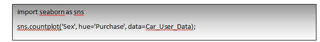
we can also check the relation between different independent variables and dependent variables by using different kinds of plots, let’s try one or two of those.
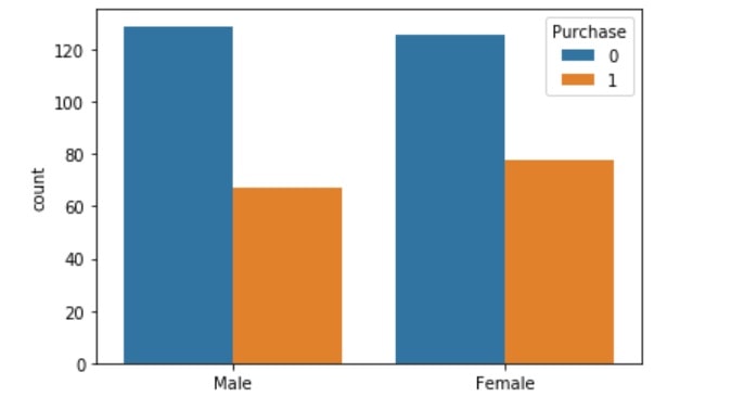
From the above image, we observe that both female and male count are almost equal, but the purchase rate of the product is slightly higher with females.

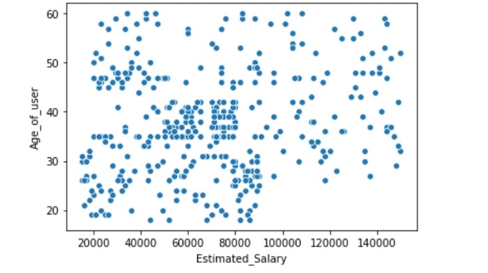
By this, above scatter plot between salary and Age we see that All age groups have low, high and medium salaried persons and observe all kinds of salaries are well scattered among different age groups. Along with plots, we can also use counts, probabilities charts and contingency tables to understand relationships between the variables.
Data Munging:
Data munging is the process of cleaning the data by handling null and outlier values. To check the nulls we can use IsNull() function with pandas data frame to know the count of null values. We already have seen that there are no null values so we need not do anything now. We can use box plots to check the outliers in different variables and handle them accordingly.
Feature Engineering:
Feature engineering is the process of choosing the correct features for the model from the data or creating new features from the available data that can capture the variance independent variables. In this use case, we are just converting the “Sex” variable which is an object data type to an integer since the algorithm handles only the integer data.
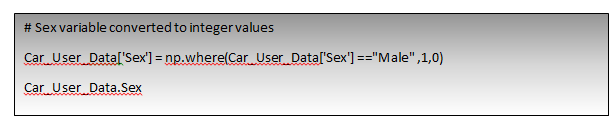
| User_ID 15624510 1 15810944 1 15668575 0 15603246 0 15804002 1 .. 15691863 0 15706071 1 15654296 0 15755018 1 15594041 0 Name: Sex, Length: 400, dtype: int32 |
Build the model:
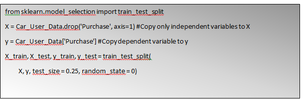
Now that every pre-processing step is done, we will move on to the model building, the first step in it would be dividing the whole dataset into train and test where we will train the model on one and test the built model on the other one.
We are using sci-kit learn library train_test_split function() to achieve this, we will be dividing the data into 75% train and 25% test.
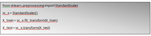
All set now, but before building model we need perform something called as standard scaling since the age and estimated salary would have different ranges, getting both of them on to the same scale would help the model to give us better predictions
Now Let us build the model using train data.
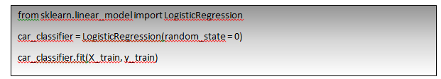
LogisticRegression(C=1.0, class_weight=None, dual=False, fit_intercept=True, intercept_scaling=1, l1_ratio=None, max_iter=100, multi_class='warn', n_jobs=None, penalty='l2', random_state=0, solver='warn', tol=0.0001, verbose=0, warm_start=False) |
Test the built model:
To test the classification model, we make use of something called as a confusion matrix, this confusion matrix will basically help us to check how well the trained model is able to classify our data(Accuracy)? i.e. how many times the actual truth(here purchase) is predicted as truth and actual false(not purchase) is predicted as false, and also few other terms which are important in use case level.
As of now let us calculate something called Accuracy of the model.
We have test set available with us already, we know the actual dependent variable we have stored it in y_test variable, now let’s predict the dependent variable from the model using X_test(independent variables) and compare the results to know how much accurate is our model.
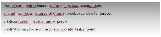
[[64 3] [ 8 25]]
Accuracy Score is: 0.89
So, from the above output, we observe that our model is performing with almost 89% accuracy on the test set which is truly amazing. In this blog, we clearly went through all concepts of logistic regression using python and also saw how it is quite different from the linear approach and its relation with linear regression. We also strongly recommend you select some classification datasets and try to build logistic regression using the above steps.

 +1 201-949-7520
 +91-9707 240 250